Linear Regression
10 Oct 2017Content:
- 1. Introduction
- 2. Least Square Approximation and Cost Function
- 3. Solving Optimization Problem
- 4. Discussion
- 5. Coding with Python
- 6. Further topics to study
- 7. Reference
1. Introduction
Suppose we have a dataset containing information of \(m\) houses which were sold in a specific area, the data contains area in meter square \((a_1)\), number of windows \((a_2)\), number of rooms \((a_3)\), and lastly, price \((b)\). We understand that \(\textbf{a}=[a_1,a_2,a_3]\) has an influence on the price of the house. Our gold is to predict the price of house providing that we have information about area, number of windows, number of rooms. This prediction is valuable because we can use predicted price to estimate the price of house we want to sell so that it will not be too high or too low regardless of the prices of all houses in the location or we can also use predicted price to determine whether the house that someone is selling is too expensive in comparision with the prices of other houses.
Linear Regression is a model to solve prediction problem. \(b\) will be expressed as a linear function of \(a_1, a_2, a_3\): \begin{equation} \tag{1}\label{eq:1} \mathbf{b}=f(\textbf{a})=x_0+x_1a_1+x_2a_2+x_3a_3 \end{equation} The problem is we cannot always find a linear relationship that fit all the data in the dataset. Our goal is to solve the linear regression problem: Find the coefficients \(\textbf{x}=[x_0, x_1, x_2, x_3]\) so that \(b\approx f(\textbf{a})\) for as much data as possible.
2. Least Square Approximation and Cost Function
Let \(\textbf{b}=[b_1, b_2,...,b_m]\) be the vector containing the value of \(m\) trainning data in dataset that we want to predict, in our example, they are \(m\) house prices.
Let \(A=[1, \mathbf{a_1} , \mathbf{a_2}, \mathbf{a_3},..., \mathbf{a_n}]\) be the matrix containing all feature data, \(\mathbf{a_1}, \mathbf{a_2},..., \mathbf{a_n}\) are column vectors containing all data of \(n\) features. In our example, \(n=3\), \(\mathbf{a_1}\) is column vector containing area in square meter of \(m\) houses, \(\mathbf{a_2}\) is column vector containing number of windows of \(m\) houses.
Let’s take a quick look at this example again:

\(A=[1, \mathbf{a_1} , \mathbf{a_2}, \mathbf{a_3}] = \begin{bmatrix}
1 & 120 & 4 & 3 \\
1 & 200 & 6 & 4 \\
1 & 80 & 2 & 2 \\
1 & 60 & 1 & 1 \\
1 & 3000 & 9 & 6
\end{bmatrix},
b = \begin{bmatrix}
10000 \\
12200 \\
70000 \\
50000 \\
19000
\end{bmatrix}\)
The linear equation \eqref{eq:1} become
\begin{equation} \tag{2}\label{eq:2}
A\mathbf{x}=\mathbf{b}
\end{equation}
It is often happens that \(A\mathbf{x}=\mathbf{b}\) has no solution. The usual reason is there are too many equations. The matrix \(A\) has more rows than columns (\(m>n\), more data the the number of features). In this case, \(b\) is a vector outside of column space of A. We cannot always get the error \(\mathbf{e}=\mathbf{b}-A\mathbf{x}\) down to zero. When \(\mathbf{e}\) is zero, \(\mathbf{x}\) is an exact solution to \(A\mathbf{x}=\mathbf{b}\). When the length of \(\mathbf{e}\) is as small as posible, \(\hat{\mathbf{x}}\) is a least square solution.
With the definition of least square solution above, the format of the cost/loss function is: \begin{equation} \tag{3}\label{eq:3} L(\mathbf{x})=||e||^2=||A\mathbf{x}-\mathbf{b}||^2_2 \end{equation}
The notation \(||\mathbf{x}||_ 2\) is Euclidean norm.If \(\mathbf{x}=(x_1, x_2,...,x_n)\) is a vector on a \(n\)-dimensional space \(R^n\) then \(||x||_ 2:=\sqrt{x_1^2+x_2^2+...+x_n^2}\). Therefore, the loss function is defined by the sum of square error: \begin{equation} \tag{4}\label{eq:4} L(\mathbf{x}) = \sum_{i=1}^{m}(\mathbf{w_i}\mathbf{x}-\mathbf{b_i})^2 \end{equation}
\(\mathbf{w_i}\) is row vector i of matrix \(A\). In our example, each \(\mathbf{w_i}\) is a row vector containing information of a house.
3. Solving Optimization Problem
The optimal \(\hat{\mathbf{x}}\) when \(A\mathbf{x}=\mathbf{b}\) has no solution is the solution of \(A^TA\hat{\mathbf{x}}=A^Tb\). The following part will be the proof of that statement.
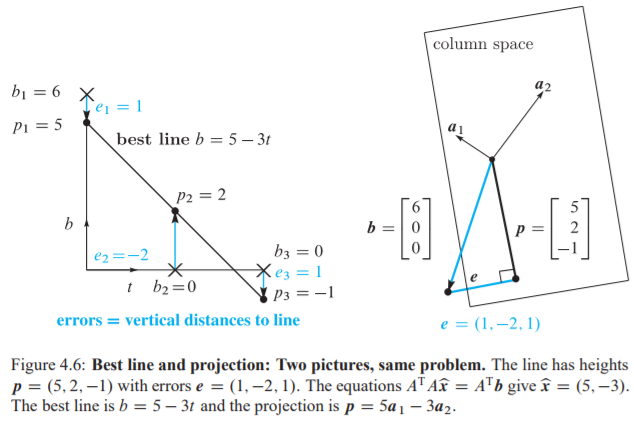
Before we move on the proof, let’s reduce the dimension of data so that it’s possible to visualize. The new problem we will solve is: Find the closest line to the points: \((0,6),(1,0),(2,0)\) or predict \(y-coordinate\) by \(x-coordinate\).
No straight line \(b=C+Dx\) goes through those three points. We are asking for two numbers C and D that satisfy three equations. Here are the equations at \(x=0,1,2\) to match the given values \(b=6,0,0\): \[C + D.0 = 6\] \[C + D.1 = 0\] \[C + D.2 = 0\] This 3x2 system has no solution because \(\mathbf{b}=[6,0,0]\) is not in the column space of matrix with 2 basis: \([1,1,1]\) and \([0,1,2]\). In other words, \(A\mathbf{x}=\mathbf{b}\) has no solution. \(A =\) \(\begin{bmatrix} 1 & 0\\ 1 & 1\\ 1 & 2 \end{bmatrix}\) , \(\mathbf{x} =\) \(\begin{bmatrix} C\\ D \end{bmatrix}\) , \(\mathbf{b} =\) \(\begin{bmatrix} 6\\ 0\\ 0 \end{bmatrix}\)
3.1. By Geometry
We are looking for a linear combination of basis of matrix \(A\), this linear combination produce a vector in the column space of \(A\) in order to minimize the length of vector \(\mathbf{e}\), \(||e||^2=||A\mathbf{x}-\mathbf{b}||^2_2\) as in equation \eqref{eq:3}. This vector \(\mathbf{e}\) is a vector from \(\mathbf{b}\) (I’m refering a vector as a point) to a point in column space of \(A\) . The smallest distance is \(\textbf{e}\) as in figure 4.6b above: \(\mathbf{e}=\mathbf{b}-\mathbf{p}\) with \(\mathbf{p}\) be the projection of vector \(\textbf{b}\) onto column space \(C(A)\).
To recap, we have proved that loss function \(L(\mathbf{x})\) is minimized when \(A\mathbf{x}\) create a projection of \(\textbf{b}\) onto column space. The formular for projection of a vector onto a subspace is: \begin{equation} \tag{5}\label{eq:5} \mathbf{p}=A(A^TA)^{-1}A^T\mathbf{b} \end{equation} The solution \(\hat{\mathbf{x}}\) is:
\begin{equation} \tag{8}\label{eq:8} \hat{\mathbf{x}} = (A^TA)^{-1}A^T\mathbf{b} \end{equation}
Proof: \(\mathbf{b}-A\mathbf{\hat{x}}\) is the error vector that is perpendicular to column space \(C(A)\). It means \(\mathbf{b}-A\mathbf{\hat{x}}\) is perpendicular to every vectors lied on \(C(A)\). Therefore, their dot product equal to 0: \(\mathbf{a_i}^T(\mathbf{b}-A\mathbf{\hat{x}})=0\) for \(i\) in range \((1,m)\). This leads to \(A^T(\mathbf{b}-A\mathbf{\hat{x}})=0\).
3.2. By Algebra
Every vector \(\mathbf{b}\) outside of column space of A can be splited into two parts. The part in column space \(\mathbf{p}\) and the perpendicular part \(\mathbf{e}\) in the nullspace of \(A^T\) (left null space of \(A\)). The reason is that column space of A (all vectors which are linear combination of column vector of matrix \(A\)) is perpendicular to left null space of \(A\) (all vectors \(\mathbf{x}\) that \(A^T\mathbf{x}=0\)). The two subspace mentioned above fill out the whole space of \(A\).
Refer to figure 4.6b, apply the law for right triangle, it stills true if the triangle lied in high dimensional space: \begin{equation} \tag{6}\label{eq:6} ||A\mathbf{x}-\mathbf{b}||^2 = ||A\mathbf{x}-\mathbf{p}||^2 + ||\mathbf{e}||^2 \end{equation} In equation \eqref{eq:6}, \(\mathbf{e}\) is a fixed vector: the error vector of projection of \(\mathbf{b}\) onto column space of \(A\). \(A\mathbf{x}-\mathbf{p}\) is a vector on column space and \(||A\mathbf{x}-\mathbf{b}||^2\) is the least square error needs to be minimized.
\begin{equation} \tag{7}\label{eq:7} ||A\mathbf{x}-\mathbf{b}||^2 = ||A\mathbf{x}-\mathbf{p}||^2 + ||\mathbf{e}||^2 \geq ||\mathbf{e}||^2 \end{equation} Since \(\mathbf{e}\) is a fixed vector, \(||\mathbf{e}||^2\) is a constant. Least square error is minimized when \(||A\mathbf{x}-\mathbf{p}||^2=0\), which means the solution \(\hat{\mathbf{x}}\) is: \begin{equation} \tag{9}\label{eq:9} \hat{\mathbf{x}}=A^{-1}\mathbf{p}=A^{-1}A(A^TA)^{-1}A^T\mathbf{b}=(A^TA)^{-1}A^T\mathbf{b} \end{equation}
3.3. By Calculus
Rewrite the term we are trying to minimized: \begin{equation} E = ||A\mathbf{x}-\mathbf{b}||^2 = (C+D.0-6)^2+(C+D.1)^2+(C+D.2)^2 \end{equation} Take partial derivative of E with respect to C and D individually: \begin{equation} \partial E / \partial C = 2(C+D.0-6) + 2(C+D.1) + 2(C+D.2) = 0 \end{equation} \begin{equation} \partial E / \partial D = 2(C+D.0-6)(0) + 2(C+D.1)(1) + 2(C+D.2)(2) = 0 \end{equation} The above system gives: \(\begin{bmatrix} 3 & 3 \\ 3 & 5 \end{bmatrix} \begin{bmatrix} C \\ D \end{bmatrix}= \begin{bmatrix} 6 \\ 0 \end{bmatrix}\) This is identical with \(A^TA\hat{\mathbf{x}}=A^T\mathbf{b}\)
In a more general case, where \(A\) is a \(m\times n\) matrix. Let’s recall the equation \eqref{eq:4} of loss function: \begin{equation} \tag{4} L(\mathbf{x}) = \sum_{i=1}^{m}(\mathbf{w_i}\mathbf{x}-\mathbf{b_i})^2 \end{equation}
In order to minimize \(L(\mathbf{x})\), we solve \(\frac{\partial L}{\partial x}=0\) for each \(x\) being element of vector \(\mathbf{x}\).
Using chain rule, the following is derivative of \(L\) with respect to \(x_1\), the first element of \(\mathbf{x}\):
\begin{equation} \tag{10}\label{eq:10} \frac{\partial L}{\partial x_1} = \sum_{i=1}^{m}2( \mathbf{w_i}\mathbf{x}-\mathbf{b_i})\mathbf{w_i}[0] \end{equation}
\(\mathbf{w_i}[0]\) is the first element of \(\mathbf{w_i}\). Notice that \(\mathbf{w_i}[0]\) for \(i\) in range \((1,m)\) is the first column of matrix \(A\), also the first row of \(A^T\). Hence, we could rewrite equation \eqref{eq:10} in matrix form:
\begin{equation} \tag{11}\label{eq:11} \frac{\partial L}{\partial x_1} = 2A^T \lbrack 0 \rbrack (A\mathbf{x}-b) \end{equation}
In equation \eqref{eq:11}, \(A^T[0]\) is first row of matrix \(A^T\). Keep going with the derivative of \(L\) with respect to every element of \(\mathbf{x}\):
\begin{equation} \tag{12}\label{eq:12} \frac{\partial L}{\partial \mathbf{x}} = 2A^T(A\mathbf{x}-\mathbf{b}) \end{equation}
In order to minimize \(L(\mathbf{x})\), the derivative in every direction is set to 0, which is \(A^T(A\mathbf{x}-\mathbf{b})=0\) which leads to the solution \(\hat{\mathbf{x}} = (A^TA)^{-1}A^T\mathbf{b}\). This is the same result as in equation \eqref{eq:8} and \eqref{eq:9}. Every approach leads to the same answer.
Note: the matrix \((A^TA)^{-1}A^T\) is also call pseudo-inverse matrix of \(A\). The notation is \(A^\dagger\) (A dagger), \(A^\dagger=(A^TA)^{-1}A^T\).
Conclusion, if \(A\) is not invertiable, the solution \(\hat{\mathbf{x}}=A^\dagger\mathbf{b}\).
4. Discussion
In the case of more than one feature, \(n>1\), column space of \(A\) become more complex (more dimension). In our example, there are 3 data points \((m=3)\), \(m\) is the dimension of the vector space that column space \(C(A)\) and \(\mathbf{b}\) lied in, more data means it’s less likely for \(\mathbf{b}\) to be lied on \(C(A)\). In this case, the solution is the projection of \(\mathbf{b}\) into \(C(A)\). Projection of a vector onto a high dimensional subspace is a vector.
4.1. Fitting a parabola
Instead of looking for coefficients \(\hat{\mathbf{x}}=[C,D]\) of the line \(b=C+Dt\), we will look for \(\hat{\mathbf{x}}=[C,D,E]\) to fit the parabola \(b=C+Dx+Ex^2\). It means the column space have one more vector: \(A= \begin{bmatrix} 1 & x_1 & x_1^2 \\ \vdots & \vdots & \vdots \\ 1 & x_m & x_m^2 \end{bmatrix}\)
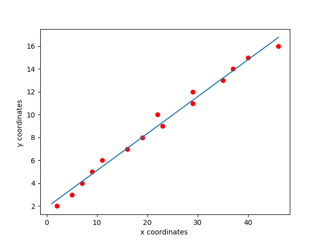
5. Coding with Python
Fit a straight line:
import numpy as np
import matplotlib
import matplotlib.pyplot as plt

# create random data
A = np.array([[2,5,7,9,11,16,19,23,22,29,29,35,37,40,46]]).T
b = np.array([[2,3,4,5,6,7,8,9,10,11,12,13,14,15,16]]).T

#Visualize data
plt.plot(A, b, 'ro')

# append column ones to matrix A
ones = np.ones((A.shape[0],1), dtype=np.int8)
A = np.concatenate((ones,A), axis=1)

# calculate coefficients to fit a straight line
A_dagger = np.linalg.inv(A.transpose().dot(A)).dot(A.transpose())
x = A_dagger.dot(b)

# start and end point of the straight line
x0 = np.linspace(1,46,2)
y0 = x[0][0] + x[1][0]*x0

# plot the straight line
plt.plot(x0, y0)
plt.xlabel('x coordinates ')
plt.ylabel('y coordinates ')
plt.show()
Using Scikit learn library
import numpy as np
import matplotlib
import matplotlib.pyplot as plt
from sklearn import linear_model

# create random data
A = np.array([[2,5,7,9,11,16,19,23,22,29,29,35,37,40,46]]).T
b = np.array([[2,3,4,5,6,7,8,9,10,11,12,13,14,15,16]]).T

#Use Scikit Learn
lr = linear_model.LinearRegression()
lr.fit(A,b)
print('Solution found by scikit learn: w =')
print(lr.intercept_) #w0
print(lr.coef_) #w1
Fitting a prabole:
import numpy as np
import matplotlib
import matplotlib.pyplot as plt

# create random data
b = np.array([[2,5,7,9,11,16,19,23,22,29,29,35,37,40,46,42,39,31,30,28,20,15,10,6]]).T
A = np.array([[2,3,4,5,6,7,8,9,10,11,12,13,14,15,16,17,18,19,20,21,22,23,24,25]]).T

#Visualize data
plt.plot(A, b, 'ro')

# append column ones to matrix A
ones = np.ones((A.shape[0],1), dtype=np.int8)
A = np.concatenate((ones,A), axis=1)

## append x^2 to A
x_square = np.array([A[:,1]**2]).T
A = np.concatenate((A,x_square), axis=1)

# calculate coefficients to fit a straight line
A_dagger = np.linalg.inv(A.transpose().dot(A)).dot(A.transpose())
x = A_dagger.dot(b)

# start and end point of the straight line
x0 = np.linspace(1,25,10000)
y0 = x[0][0] + x[1][0]*x0 +x[2][0]*x0*x0

# plot the parabola
plt.plot(x0, y0)
plt.xlabel('x coordinates ')
plt.ylabel('y coordinates ')
plt.show()

This parabole seems to be underfitting. We need to make the regression equation more complex by adding features (add more dimension to \(C(A)\)).
6. Further topics to study
- Evaluation approach such as cross-validation (Determine which solution is the best)
- Normalization, data value could be in different scale and causing inconsistent.
- Regularization to avoid overfitting.
7. Reference
- Introduction to Linear Algebra book by Prof. Gilbert Strang.
- Andrew, Ng. , ‘Machine learning’, Standford University Online, lecture notes week 2, [online]: https://www.coursera.org/learn/machine-learning