K-Means Clustering with Visualization tool

Content:

• 1. Objective
• 2. Introduction
• 3. Mathematical Analysis
  • 3.1. Input and Output
  • 3.2. Lost Function and Optimization Problem
  • 3.3. Solving Optimization Problem
    • 3.3.1. Fixed \(\mathbf{M}\), center of observation group
    • 3.3.2. Fixed \(\mathbf{Y}\), label vector of each observation
  • 3.4. Algorithm Summary and Flowchart
    • 3.4.1. Summary
    • 3.4.2. Flowchart
  • 3.5. Discussion
    • 3.5.1. Convergence
    • 3.5.2. Sensitiveness to initial cluster
• 4. Application in Data Compression
• 5. Conclusion
• 6. Acknowledgement
  • 6.1. Reference
• 7. Source Code and PDF report
  • 7.1. Declare Data types

1. Objective

After reading this blog, you will be able to

1. Understand a clustering method (unsupervised learning) namely K-means algorithm from mathematical perspective.
2. Source code of visualization tool (written in Pascal), demo below.
3. Source code of image compression, image segmentation tool, applied K-Means Algorithm (written in Pascal).

1.1. Abstract

Clustering problem is a task of dividing a set of objects (also called members) into different groups (called clusters) based on object’s characteristics. Members of a group will have more similarities in comparison with those in other group. This report discusses a traditional clustering method called K-Means algorithm from mathematical perspective. Additionally, an experiment is provided to examine the algorithm in two dimensional space then an application in image compressing.

2. Introduction

Clustering problems arise in many different applications: machine learning data mining and knowledge discovery, data compression and vector quantization, pattern recognition and pattern classification.

The goal of K-Means Algorithm is to correctly separating objects in a dataset into groups based on object’s properties. For instance, objects could be house and their properties are size, number of floor, location, power consumption per year, etc. The goal is to classify house dataset into groups which are luxury, average, poor. In that case, all properties of houses have to be processed to turn into number to create a vector, this process is called vectorization.

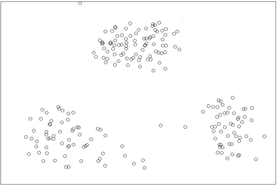
Another example, take each points in a panel as a objects and each object has two properties which are x-axis and y-axis location, with input \(K=3\). The algorithm correctly finds the cluster (fig 1).

Fig 1: Running K-means algorithm to find 3 cluster

3. Mathematical Analysis

3.1. Input and Output

The K-Means Algorithm takes a set of observations \(X=[x_1,x_2,...,x_N]\) \(\in\) \(R^{d \times N}\) where each observation is a \(d\)-dimensional vector, \(N\) is the number of observations (members) and the number of group \((K, K<N)\) as two input. The algorithm outputs the center of \(K\) group \([m_1,m_2,...,m_K] \in R^{d \times K}\) and the index or name of group that each member belonged to (label of the group).

3.2. Lost Function and Optimization Problem

Suppose \(x_i\) \((i\in[1,N])\) belong to cluster \(k\) \((k \in [1,K]\), the lost value of observation \(x_i\) is the distance from observation \(x_i\) to center \(m_k\) in euclidean space, defined by \((x_i-m_k)\). Let’s \(y_i=[y_{i1},y_{i2},...,y_{iK}]\) be the label vector of each observation \(x_i\), \(y_{ik}=1\) if \(x_i\) belongs to group \(k\) and \(y_{ij}=0\) \(\forall j\neq k\). Label vector of each observation contains only one digit \(1\) because each observation belongs to only one group which leads to the following equation. \begin{equation} \tag{1}\label{eq:1} \sum_{k=1}^{K} y_{ik} = 1 \end{equation} The objective is to minimize the within-cluster sum of squares (variance), also known as square errors of, where each square error of an observation \(x_i\) from group \(m_k\) is defined by: \begin{equation} \tag{2}\label{eq:2} ||x_{i}-m_{k}||^2=y_{ik}||x_{i}-{m_k}||^2 \end{equation} From the equation \eqref{eq:1}, sum of all elements in a label vector is equal to 1. The square error of an observation is: \begin{equation} \tag{3}\label{eq:3} y_{ik}||x_{i}-{m_k}||^2=\sum_{j=1}^{K}y_{ij}||x_{i}-m_{j}||^2 \end{equation} The square error of all observation is the sum of every square error of in the given set of observation. The goal is minimize the lost function, equation \eqref{eq:4} where \(Y=[y_1,y_2,...,y_N]\) be the matrix contains all label vector of \(N\) observation and \(M=[m_1,m_2,...,m_K]\) be the center of \(K\) groups (clusters). \begin{equation} \tag{4}\label{eq:4} f(Y,M)=\sum_{i=1}^{N}\sum_{j=1}^{K}y_{ij}||x_i-m_j||^2 \end{equation} The objective is also to find the center and label vector of each observation which are Y and M, the two outputs that are mentioned in input and output. \begin{equation} \tag{5}\label{eq:5} Y,M=argmin_{Y,M}\sum_{i=1}^{N}\sum_{j=1}^{K}y_{ij}||x_i-m_j||^2 \end{equation}

3.3. Solving Optimization Problem

There are two variable in equation \eqref{eq:5} which are center of each group of observation and label vector of each observation. The problem could be solved by fixed each variable then minimize the other variable.

3.3.1. Fixed \(\mathbf{M}\), center of observation group

Because all centers (\(M\)) are constant, the objective is to correctly identify label vector which is identifying the group that each observation belonged to so that the square error in equation \eqref{eq:4} is minimized. \begin{equation} \tag{6}\label{eq:6} y_i = argmin_{y_i}\sum_{j=1}^{K}y_{ij}||x_i-m_j||^2 \end{equation} Retrieving from equation \eqref{eq:1}. Because only one element in vector \(y_i\) \(i\in[1,K]=1\). Equation \eqref{eq:6} could be rewritten as: \begin{equation} \tag{7}\label{eq:7} j=argmin_{j}||x_i-m_j]]^2 \end{equation} The value of \(||x_i-m_j||^2\) is the square of distance from observation to center of group in euclidean space. Concretely, when M is constant, equation \eqeqref{eq:7} shows that minimizing the sum of square error could be achieved by choosing label vector so that the center are closest to observation.

3.3.2. Fixed \(\mathbf{Y}\), label vector of each observation

When label vector (\(Y\)) are constant, the objective is to correctly identify the center so that the square error in equation \eqref{eq:4} is minimized. In this case, the optimization problem in equation \eqref{eq:5} could be rewritten by the following equation. \begin{equation} \tag{8}\label{eq:8} m_j=argmin_{m_j}\sum_{i=1}^{N}y_{ij}||x_i-m_j||^2 \end{equation} The equation \eqref{eq:8} is a convex function and differentiable for each \(i\in[1,N]\). Hence equation \eqref{eq:8} could be solved by finding the root of the partial derivative function. This approach will make sure that the root is the the value that make the function reach a optimum. Let’s \(g(m_j)=\sum_{i=1}^{N}y_{ij}||x_i-m_j||^2\) (retrieving from equation \eqref{eq:8} and take the partial derivative of \(g(m_j)\): \begin{equation} \tag{9}\label{eq:9} \frac{\partial g(m_j)}{\partial m_j}=2 \sum_{i=1}^{N}y_{ij}(m_j-x_i) \end{equation} The equation \eqref{eq:9} is equal 0 is equivalent to: \begin{equation} \tag{10}\label{eq:10} m_j\sum_{i=1}^{N}y_{ij}=\sum_{i=1}^{N}y_{ij}x_{i} \end{equation} \begin{equation} \tag{11}\label{eq:11} \Leftrightarrow m_j=\frac{\sum_{i=1}^{N}y_{ij}x_{i}}{\sum_{i=1}^{N}y_{ij}} \end{equation} The value of \(y_{ij}=1\) when observation \(x_i\) belongs to group \(m_j\). Hence, the denominator of equation \eqref{eq:11} \(\sum_{i=1}^{N}y_{ij}\) is the number of observations that belonging to group \(m_j\) and the nominator \(\sum_{i=1}^{N}y_{ij}x_{i}\) is the sum of all observations belonging to group \(m_j\). In other word, when Y is constant, the square errors could be minimize by assigning the centers to the means of observations in the groups that the observations belonging to.

3.4. Algorithm Summary and Flowchart

3.4.1. Summary

The algorithm can be done by continuously constantize Y and M, one each a time as discussed in Fixed \(M\)and Fixed \(Y\).

Step 1. Select K points as cluster centers randomly. (K is the number of group/cluster)
Step 2. Assign all data points to corresponding cluster center created in step 1 based on Euculidean distance.
Step 3. Move cluster center, new cluster centers are means of coordination of all data points among same group.
Step 4. Repeat step 2 until convergence (when all cluster centers remain unchanged after an iteration).
Step 5. Clustering process is done, if we have new data points, caculate distance between that data point to the cluster centers that we found and see what group the data point belongs to.

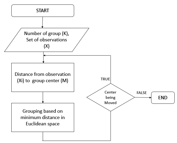
3.4.2. Flowchart

The following chart describe K-Means Algorithm.

Fig 2: K-Means Algorithm Flowchart

3.5. Discussion

3.5.1. Convergence

The algorithm will stop after a certain number of iteration because the square error function is a strictly decreasing sequence and the square error is always greater than 0. But this algorithm will not make sure that it will find a global optimum because solving the equation \eqref{eq:8} by finding the root when the partial derivative is equal 0 will only return the value for local optima but not make sure that local optima will be a global minimum. The following figure describe a case where poorly seeding leads to a local optimum.

Fig 3: Poorly seeded leads to inaccurate result

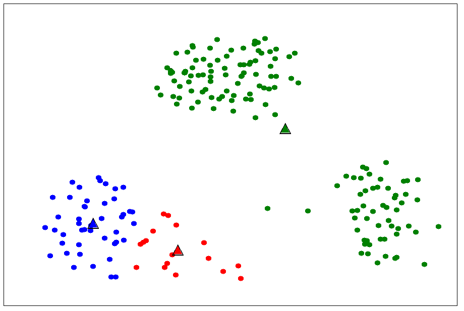
This result leads to a very high square error compared to the result in fig 1.

3.5.2. Sensitiveness to initial cluster

K-Means algorithm requires careful seeding, which means the final result is very sensitive to the initial value of cluster. Numerous efforts have been made to improving K-Means clustering algorithm due to its drawbacks \(^[2]\).

4. Application in Data Compression

Left image: 900 KB, Right image (K=16 color): 70KB

More detail will be described in the upcomming blog Image Compression

5. Conclusion

K-Means Algorithm could be very simple and quick to be implemented, the clustering problems where all clusters are centroids and separated can be solved by the algorithms.

This report doesn’t come with new idea to improve the effectiveness of the algorithm, the aim of the report is to introduce the readers to a basic clustering method with some visual examples on 2-dimensional and 3-dimensional data.

6. Acknowledgement

The ideal of K-means Algorithm is leaned by me from Machine Learning course by Prof. Andrew Ng from coursera.

The mathematical approach to solve the optimization problem is learned by me from the article on K-means algorithm (machine learning fundamental) by Tiep Vu.

6.1. Reference

[1]. Joaqun Prez Ortega, Ma. Del, Roco Boone Rojas, and Mara J.Somodevilla “Research issues on k-means algorithm: An experimental trial using matlab”.

[2]. Arthur,~D.,~Vassilvitskii,~S., 2016. k-Means++: The Advantages of Careful Seeding, Technical Report, Stanford.

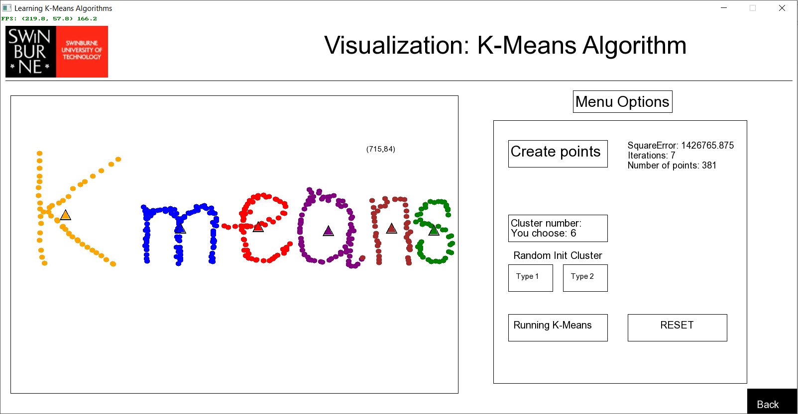
7. Source Code and PDF report

This part will guide you through all the code in this program, if you understand the algorithm, you could implement it on any programming language not just pascal. With a click of a button, all characters are separated using K-means algorithm, the program will look like this:

Program interface

7.1. Declare Data types

const
  POINT_RADIUS = 5;
  X_DIFF = 20; //location panel and point location
  Y_DIFF = 160; //location panel and point location

type    
  // type used for application  
  RGB = array[0..2] of Single; // x-axis  // store red, green and blue of an image
  CollumnPixels = array of RGB; // y-axis, rowPixels
  imgArray = array of CollumnPixels; // 3-dimensional array used to store red, green, blue color of each pixel in an image 
  IntArray = array of Integer; // label

  SingleColorArray = array of Color; // 1 dimensional array used to store color
  ColorArray = array of SingleColorArray; // 2 dimensional array used to store color
  
  // typed used for Visualization
  PointsRecord = Record
    x    : Single; // x-axit on panel
    y    : Single; // y-axit on panel
    idx  : Integer; // store label of each point, instead of create another array or enumeration to store it
  end;

  PointsArray = array of PointsRecord; // Store all the points on panel and the init points

In the panel, each point’s data type is PointsRecord, it has x and y properties, they are the x-axis and y-axis of each point, idx is the label of each point, idx keep changing overtime during the iterations.

Continue Reading… Please download source code!

Download PDF Report Full code in Pascal: https://github.com/DungLai/Image-Compression-Segmentation