Gradient Descent
21 Dec 2017An optimization algorithm which uses gradient value of cost function to recursively adjust the solution of optimization problem.
Content:
1. Introduction
1.1. Why gradient descent?
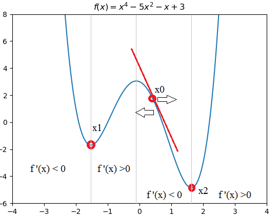
Given an optimization problem: Find \(x\) so that \(f(x)=x^4-5x^2-x+3\) as in figure 1 reaches minumum value, an approach is to solve \(f'(x)=0\) to find all local minima then compare them to get global minimum. In our example, solving \(f'(x)=0\) gives us 2 local minima at \(x=x_1\) and \(x=x_2\), because \(f(x_1)>f(x_2)\) hence \(f(x)\) reaches minimum at \(x=x_2\).
The problem with the approach above is that sometimes, the equation \(f'(x)=0\) cannot be solved easily. In this case, we can use an algorithm call gradient descent to find the approximate solution.
1.2. Methodology
To be more specific, GD will iteratively change the value of \(x\) \((x:=x+\beta)\) so that in each iteration, hopefully, \(f(x)\) is getting smaller and moving closer to the minimum.
One way to ensure that the adjustment \(\beta\) to \(x\) will cause \(f(x)\) smaller is to make \(\beta\) equal a portion of the negative of the gradient: \(\beta=-\alpha f'(x)\) where \(\alpha\) is a positive number and it’s called learning rate. In conclusion, the adjustment to \(x\) will be:
\begin{equation} \tag{1} \label{eq:1} x := x - \alpha f’(x) \end{equation}
Considering the point \(x_0\) in figure 1, because \(f'(x0)<0\) so \(\alpha f'(x) <0\) which means the update to \(x\) as in equation (\ref{eq:1}) will move \(x\) to the right hand side, making \(f(x)\) descending.
2. Gradient Descent for Linear Regression
Before we move on to the implementation and visualization, let’s quickly go through the concept of matrix derivative (to work with multi-dimensional data) and numerical differentiation (to calculate approximate gradient at a specific value of \(x\))
2.1. Matrix derivatives
In our previous example, \(x\) is one-dimensional vector, but it’s not likely the case in most problem, \(x\) could a vector in n-dimensional space. In this case, we need to update all element in \(x\) simutaneously. If we don’t update them simutaneously then \(f'(x)\) will change everytime an element in \(x\) is updated. Matrix derivatives could help us archieve that.
The following equation is the formula for derivatives of \(f(A)\) with respect to \(m\)x\(n\) matrix \(A\).
\begin{equation} \triangledown_A f(A) = \begin{bmatrix} \frac{\partial f}{\partial A_{11}} & \cdots & \frac{\partial f}{\partial A_{1n}} \newline \vdots & \ddots & \vdots \newline \frac{\partial f}{\partial A_{m1}} & \cdots & \frac{\partial f}{\partial A_{mn}} \end{bmatrix} \end{equation}
In linear regression, \(x\) is a vector. Formula for derivatives with repsect to a vector:
\begin{equation} \triangledown_x f(x) = \begin{bmatrix} \frac{\partial f}{\partial x_{1}}\newline \vdots \newline \frac{\partial f}{\partial x_{m}} \end{bmatrix} \end{equation}
2.2. Numerical Differentiation
Numerical Differentiation can be used to check whether our gradient function (in code) is correct or not. When testing, give some value \(x\) then check whether or not \(f'(x)\) calculated by equation \eqref{eq:2} is closed enough to \(f'(x)\) calculated by equation \eqref{eq:3}. \begin{equation} \tag{2} \label{eq:2} f’(x) = \lim_{\varepsilon \rightarrow 0}\frac{f(x + \varepsilon) - f(x)}{\varepsilon} \end{equation}
\begin{equation} \tag{3} \label{eq:3} f’(x) \approx \frac{f(x + \varepsilon) - f(x - \varepsilon)}{2\varepsilon} \end{equation}
The proof of numerical differentiation can be found at Wikipedia
2.3. Python code for visualization
import numpy as np
import matplotlib
import matplotlib.pyplot as plt
from sklearn import linear_model
import matplotlib.animation as animation
import os
import subprocess

# apply gradient descent algorithm to optimiza cost function of several variables

def cost(x):
	"""Cost function of linear regression (LR) model with coefficient x"""
	m = A.shape[0]
	return .5/m *np.linalg.norm(A.dot(x)-b,2)**2

def grad(x):
	"""Gradient function of cost function"""
	m = A.shape[0]
	return 1/m *A.T.dot(A.dot(x)-b)

def numerical_grad(x, cost):
	"""Calculating numerical gradient with coefficient x to check whether our grad function is correct or not"""
	eps = 1e-4
	g = np.zeros_like(x)
	for i in range(len(x)):
		x_p = x.copy()
		x_n = x.copy()
		x_p[i] += eps
		x_n[i] -= eps
		g[i] = (cost(x_p) - cost(x_n))/(2*eps)
	return g

def check_grad(x, cost, grad):
	"""Check grad function by comparing actual gradient value and numerical gradient (estimation)"""
	x = np.random.rand(x.shape[0], x.shape[1])
	grad1 = grad(x)
	grad2 = numerical_grad(x, cost)
	return True if np.linalg.norm(grad1 - grad2) < 1e-6 else False

def gradient_descent(x_init, grad, alpha):
	"""
	Running gradient descent with initial value x_init, grad function, learning rate alpha
	This function return x: list of solution after each iteration and iteration: last iteration it has gone through
	"""
	m = len(x_init)
	x = [x_init]
	for iteration in range(itr):
		x_new = x[-1] - alpha*grad(x[-1])
		if np.linalg.norm(grad(x_new))/m < 1e-3: #Stop gradient descent when grad value is too small.
			break
		x.append(x_new)
	return (x, iteration)

############### Main ####################

# create random data
A = np.array([[2,9,7,9,11,16,25,23,22,29,29,35,37,40,46]]).T
b = np.array([[2,3,4,5,6,7,8,9,10,11,12,13,14,15,16]]).T

fig1 = plt.figure('GD for Linear Regression')
ax = plt.axes(xlim=(-10, 60), ylim=(-1, 20)) #restrict the figure showing only values in specified range
plt.plot(A,b,'ro', label='_nolegend_') # plot data points
line, = ax.plot([], [], color = 'blue') # plot function used in animation

# plot solution found by scikit learn
lr = linear_model.LinearRegression()
lr.fit(A,b)
x0_gd = np.linspace(1,46,2)
y0_sklearn = lr.intercept_[0] + lr.coef_[0][0]*x0_gd
plt.plot(x0_gd, y0_sklearn, color='green')

# apply gradient descent
itr = 90
learning_rate = .0001 #.0001
x_init = np.array([[1], [2]])

ones = np.ones((A.shape[0],1), dtype=np.int8) #Append bias to A
A = np.concatenate((ones,A), axis=1)

print('Checking gradient...', check_grad(np.random.rand(2, 1), cost, grad)) #Output: Checking gradient... True

x_init = np.array([[1], [2]])

# running gradient descent
myGD = gradient_descent(x_init, grad, learning_rate)

# plot x_init (black line)
x0_gd = np.linspace(1,46,2)
y0_init = x_init[0][0] + x_init[1][0]*x0_gd
plt.plot(x0_gd, y0_init, color = 'black')

# plot lines in each iteration
def update(i):
	x_gd = myGD[0][i]
	y0_gd = x_gd[0][0] + x_gd[1][0]*x0_gd
	line.set_data(x0_gd,y0_gd)
	plt.xlabel('Iteration: {}/{}, learning rate: {}'.format(i+1, myGD[1], learning_rate))
	return line,

# legend for graph
plt.legend(('Value in each GD iteration', 'Solution by formular', 'Inital value for GD'), loc=(0.52, 0.01))
ltext = plt.gca().get_legend().get_texts()
plt.setp(ltext[0], fontsize=10)
plt.setp(ltext[1], fontsize=10)
plt.setp(ltext[2], fontsize=10)

# save animation to mp4 file using ffmpeg
Writer = animation.writers['ffmpeg']
writer = Writer(fps=15, metadata=dict(artist='Me'), bitrate=1800)

line_ani = animation.FuncAnimation(fig1, update, myGD[1]+1, interval=50, blit=True)
# # Save mp4 file for animation, require ffmpeg and set path to environment variable.
# line_ani.save('lines.mp4', writer='ffmpeg')

# # Convert mp4 to gif
# # https://stackoverflow.com/questions/11269575/how-to-hide-output-of-subprocess-in-python-2-7
# FNULL = open(os.devnull, 'w')
# subprocess.call(['ffmpeg', '-i', 'lines.mp4', 'lines.gif'], stdout=FNULL, stderr=subprocess.STDOUT) # Execute command line to convert .mp4 to .gif using ffmpeg and hide output of command line to terminal
plt.show()

plt.figure('Iter and cost function')

cost_list = []
iter_list = []

for i in range(itr):
	iter_list.append(i+1)

for i in range(itr):
	cost_list.append(cost(myGD[0][i]))

plt.plot(iter_list, cost_list)
plt.xlabel('Iteration')
plt.ylabel('Cost value')

plt.show()
3. Discussion
3.1. When to stop?
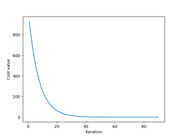
The relationship between cost value in each iteration is shown in figure 2.a, clearly, the cost value tends to bottoms out and remains stable after iteration 40. The rest iteration doesn’t seem to reduces the cost value as much and could be unnecessary. When the calculation is expensive, we might not want to continued the iteration while the solution is already good enough. So plotting cost value after each iteration or even calculating the slope of that function could be a way to decide when to stop GD.
Figure 2.b shows that setting \(1e-3\) as the threshold is not good enough to stop GD because in that example, the optimal solution occurs when \(\mid {grad} \mid \approx 5.94\).
3.2. Stucking in Local Optimum
In figure (3), when trying to fit data by a parabola, GD get stuck in a local optimum, we know that because the green line is the solution found by formula (which is global optimum as I have explain in this blog). When trying to fit a parabola, another vector is added to the collumn space. When working with high dimensional space, it’s likely to have multiple local mimima. It means GD is very sensitive to initial value and it’s hard to get out of a local minimum. There are serveral variant of GD that can deal with this problem such as Stochastic Gradient Descent.
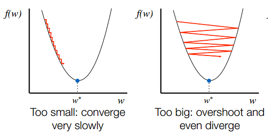
3.3. Speed to convergence (Learning rate)
Learning rate (\(\alpha\)) is an important parameter, small learning rate as in figure 4.a can slow down GD and maybe makes it very slow to converge. On the other hand, large learning rate as in figure 4.b can make GD impossible to converge.
3.4. Disadvantage compared to using formula
| Gradient Descent | Normal Equation |
|---|---|
| Need to chose learning rate | No need to choose learning rate |
| Needs many iteration | Don’t need to iterate |
| Work well even when n (features) is large | Need to compute projection matrix 0(n3) |
| O(kn2) | Slow if n (features) is very large |
3.5. Speedup GD
Feature Scaling is commonly be used when working with GD, we want features are in similar scale (range) and it can be archieved by:
- Rescaling: The simplest method is rescaling the range of features to scale the range in [0, 1] or [−1, 1]. Selecting the target range depends on the nature of the data.
\begin{equation} x’=\frac{x-min(x)}{max(x)-min(x)} \end{equation}
\(x\) is original value and \(x'\) is the normalized value.
- Mean normalisation
\begin{equation} x’=\frac{x-mean(x)}{s_i} \end{equation}
\(s_i\) can be standard deviation or \(s_i\) is the range of value (max-min).