Singular Value Decomposition

Content:

• Diagonalize
• SVD
• Image Compression using SVD
• Reference

Diagonalize

If a matrix \(A\) can be diagonalized by matrix \(P\): \begin{equation} P^-1AP = \begin{bmatrix} \tag{1}\label{eq:1} \lambda_1 & & & \newline & \lambda_2 & & \newline & & \ddots & \newline & & & \lambda_n \end{bmatrix} \end{equation} then:

\begin{equation} \tag{2}\label{eq:2} AP = P \begin{bmatrix} \lambda_1 & & & \newline & \lambda_2 & & \newline & & \ddots & \newline & & & \lambda_n \end{bmatrix} \end{equation}

Let’s \(p_i\) be collumn vectors of matrix \(P\): \begin{equation} \tag{3}\label{eq:3} P = ( \vec{p_1} \hspace{2em} \vec{p_2} \hspace{2em} … \hspace{2em} \vec{p_n}) \end{equation}

Equation \eqref{eq:2} can be rewritten as \(A \vec{p_i} = \lambda_i \vec{p_i} \hspace{1.2em} (i=1,2,...,n)\)

So the column vectors of \(P\) are right eigenvectors of \(A\), and the corresponding diagonal entry is the corresponding eigenvalue. The invertibility of \(P\) also suggests that the eigenvectors are linearly independent. This is the necessary and sufficient condition for diagonalizability and the canonical approach of diagonalization. The row vectors of \(P^{-1}\) are the left eigenvectors of \(A\).

A matrix is diagonalizable if P is invertible: all eigenvectors are linearly independent.

Check for nondiagonalizable matrices:

1. Calculate geometric multiplicity (GM): The number of independent eigenvectors.
2. Calculate algebraic multiplicity (AM): The number of repeated \(\lambda\).
3. GM < AM => nondiagonalizable

This is “spectral theorem” or “principle axis theorem”: For every symetric matrix A, \begin{equation} A = QDQ^{-1} = QDQ^T \hspace{2em} with \hspace{1em} Q^{-1} = Q^T \end{equation}

(Proof [1] page 331)

SVD

The singular value decomposition of a matrix A is the factorization of A into the product of three special matrices: \(A=U \sum V^T\) where \(U\) and \(V\) are square orthonormal and the matrix \(\sum\) is diagonal with positive real entries in the main diagonal.

The number of non-zero entries on matrix \(\sum\) is the rank of matrix \(A\).

The diagonal entries of \(\sum\) are sorted from biggest to smallest.

Image Compression using SVD

An image can be factorized into the multiplication of 3 matrices using SVD technique. The diagonal matrix is called the energy of the image.

Figure 1: a) Test image b) Entries in diagonal matrix after SVD factorization

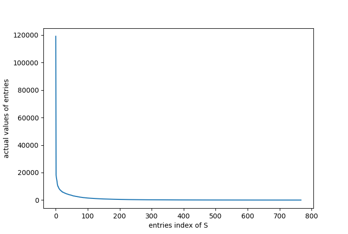
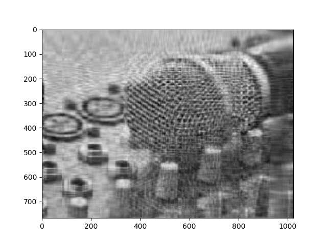
Figure b below shows that most values of those entries are closed to zero, that means these values will not contribute much to the overall image, the first 100 values will significantly affect the structure of the image. The following figure show the compressed image by only retaining the first 50 values of S. This method is called “best rank k approximation”.

Figure 2: a) k=20 b) k=50

import scipy
from scipy import misc
from scipy import linalg
import numpy as np
import math
import matplotlib
from matplotlib import pyplot as plt

# load image test.png and store pixel values in matrix A
# Dimesional of image (1024x768)
A = scipy.misc.imread('test.png', mode='L')

U,S,V = linalg.svd(A, full_matrices = True)
plt.figure(1)
plt.imshow(A,cmap='gray')

# Plot the values of entries in diagonal matrix S
plt.figure(3)
fig, ax = plt.subplots()
plt.plot(S)
ax.set(xlabel='entries index of S', ylabel='actual values of entries')

# k is the number of largest entries on diagonal matrix that will be retained
k = 50
S[k:] = 0

n=1024
m=768
sigma = np.zeros((m, n))
for i in range(min(m, n)):
	sigma[i, i] = S[i]

A = np.dot(U, np.dot(sigma, V))

plt.figure(2)

# Plot image after choosing k biggest entries of S
plt.imshow(A,cmap='gray')

plt.show()

Reference

1. Introduction to linear algebra 4th edition, Gilbert Strang.